Forecasting is rarely about guessing the future. In practice, it is about learning the rhythm of the past and using that rhythm to make disciplined, defensible predictions. Time series data, such as daily orders, monthly revenue, website visits, or electricity demand, often contains repeating patterns and long-term movement that can mislead teams if analysed as a single stream. Time series decomposition helps by separating the series into meaningful components: trend (the long-run direction), seasonality (regular cycles), and residuals (random noise). Once these parts are understood, forecasting models such as ARIMA and Exponential Smoothing can be applied more accurately. This approach is widely taught and practised in business analytics classes because it turns raw time-based numbers into decisions that can be explained and improved.
Why Decomposition Matters Before Forecasting
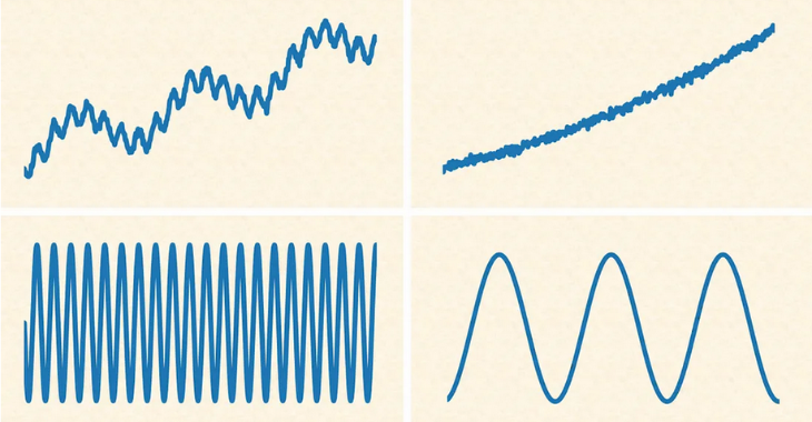
A time series can look chaotic at first glance. Sales rise, fall, spike during festivals, drop during holidays, and shift during market changes. Decomposition acts like a careful lens that breaks the signal into distinct layers.
Trend: the underlying movement
Trend captures the general direction over time. For example, a subscription product may show steady growth due to expanding customer adoption. Without isolating the trend, short-term fluctuations can hide the real business trajectory.
Seasonality: repeated cycles
Seasonality is not random. It is predictable repetition, such as higher retail demand during weekends, peak bookings during summer, or payroll-related spending at month’s end. Identifying this pattern helps avoid overreacting to expected fluctuations.
Residual: what remains unexplained
Residuals contain irregular movements not captured by trend and seasonality. These can include one-time promotions, outages, supply chain disruptions, or sudden news-driven demand. Residual analysis is valuable because it highlights unusual events that may require separate treatment.
Decomposition is not a model by itself. It is a preparation step that improves model choice, diagnostics, and stakeholder confidence.
Common Decomposition Methods and When to Use Them
Decomposition can be performed using additive or multiplicative assumptions.
Additive decomposition
This assumes components add together:
Observed = Trend + Seasonality + Residual
It works well when seasonal swings stay roughly constant over time, such as a stable weekly traffic pattern.
Multiplicative decomposition
This assumes components multiply:
Observed = Trend × Seasonality × Residual
It is better when seasonal variation grows as the trend increases, such as revenue seasonality increasing as the business scales.
In real projects, the choice depends on how the seasonal amplitude behaves over time. A quick visual check often provides the first clue, and model diagnostics confirm it.
ARIMA Forecasting After Understanding Components
ARIMA is a classic forecasting model that performs well when a time series can be made stationary, meaning its statistical properties remain stable over time after transformations.
What ARIMA captures
ARIMA combines three ideas:
- AR (AutoRegressive): current values depend on past values
- I (Integrated): differencing removes trend to stabilise the series
- MA (Moving Average): current values depend on past forecast errors
In practical terms, ARIMA works well when trend and autocorrelation dominate, and when you can apply differencing to remove long-run movement. Seasonality can be handled using a seasonal variant called SARIMA, which extends ARIMA to model repeating cycles explicitly.
When ARIMA is a good fit
ARIMA is useful when:
- the series has strong autocorrelation
- you can justify stationarity through differencing
- the goal is a statistically grounded forecast with clear diagnostics
However, ARIMA demands careful parameter selection and validation. It is not a “plug-and-play” option. Teams typically confirm model fitness using residual checks, autocorrelation plots, and forecast error metrics.
Exponential Smoothing for Practical, Robust Forecasts
Exponential Smoothing models focus on weighted averages, giving more importance to recent observations. They are often preferred for operational forecasting because they are intuitive, efficient, and strong in many real-world datasets.
Key variants
- Simple Exponential Smoothing: best for data with no trend or seasonality
- Holt’s Linear Trend Method: handles trend
- Holt-Winters (Triple Exponential Smoothing): handles both trend and seasonality
Holt-Winters is especially useful when seasonality is strong and stable, such as recurring monthly demand cycles. It can be implemented in additive or multiplicative forms, aligning naturally with decomposition thinking.
Why teams use it often
Exponential Smoothing is popular because:
- it adapts quickly to recent changes
- it handles trend and seasonality without heavy statistical requirements
- it produces reliable baselines for planning and inventory decisions
In many forecasting tasks, a well-tuned Holt-Winters model can rival more complex approaches, particularly when the patterns are consistent and explainable.
Model Selection, Validation, and Forecast Quality
Choosing between ARIMA and Exponential Smoothing is not about which is “better” in theory. It depends on the data behaviour and the business need. A strong practice is to benchmark both.
Good validation habits
- split data into training and test windows
- use metrics such as MAE, RMSE, or MAPE depending on business sensitivity
- check residuals for patterns, which may indicate missing seasonality or structural changes
- monitor forecast stability over time rather than trusting a one-time result
This disciplined workflow is a core reason forecasting is repeatedly taught in business analytics classes, because organisations need forecasts that are not only accurate but also defensible and maintainable.
Conclusion
Time series decomposition and forecasting work best when treated as a structured process rather than a quick model run. By separating trend, seasonality, and residual components, teams gain clarity about what drives changes over time and avoid misleading interpretations. ARIMA provides a statistically rigorous approach for autocorrelated series, while Exponential Smoothing offers a practical and adaptable method for operational planning. When combined with sound validation and continuous monitoring, these techniques can produce forecasts that support smarter inventory control, staffing, budgeting, and demand planning decisions.